機械学習｜Pythonかんたん環境構築からのAI入門

環境の構築と実際の運用

• Google Colaboratory
• VMware での 仮想環境
• Windows と Linux の デュアルブート

関連記事

機械学習による競輪予想

Google Colaboratory

Google Driveとの連携にプログラムを書かなくてよくなったため、ローカルとGoogle Colaboratory上のプログラムに差を作らなくていいので、私的には楽になりました。

Google Colaboratory

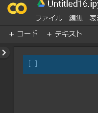
ドライブをマウント を 選択

from sklearn.svm import SVC
from sklearn.metrics import accuracy_score
import tensorflow as tf
import numpy as np
import pandas as pd

＃GPUの利用 keras用だったはず　故にいらない。
config = tf.ConfigProto()
config.gpu_options.per_process_gpu_memory_fraction = 0.8
sess = tf.Session(config=config)
K.set_session(sess)

データの前処理パートがここに入る

Answer to the Ultimate Question of Life, the Universe, and Everything
＝42
だからrandom_state=42となる。

clf = SVC(kernel='linear', random_state=42, gamma='scale')
clf.fit(X_train,y_train)
y_pred = clf.predict(X_test)

print(accuracy_score(y_test,y_pred))

########################################################################
#####SVC grid
########################################################################
Cs = [0.0001,0.01,0.1,1,10]
gammas = [0.0001,0.01,0.1,1,10]
param_grid = dict(svc__gamma=gammas, svc__C=Cs)
cv = StratifiedShuffleSplit(n_splits=5, test_size=0.2, random_state=42)
#cv=10

svm_set = Pipeline([('scaler', StandardScaler()),('svc',SVC())])
grid = GridSearchCV(svm_set, param_grid=param_grid, cv=cv)

grid_result = grid.fit(X, y)
print("Best: %f param %s" % (grid_result.best_score_, grid_result.best_params_))

grid_result = grid.fit(X_test, y_test)
print("Best: %f param %s" % (grid_result.best_score_, grid_result.best_params_))

result_dic = grid_result.best_params_
svc__C_value =  result_dic["svc__C"]
svc__gamma_value =  result_dic["svc__gamma"]


clf = SVC(kernel='linear', random_state=42, gamma=svc__gamma_value,probability=True,C=svc__C_value)
clf.fit(X, y)
df_test = df_test.fillna(0)
predict_data = clf.predict(df_test)

predict_data = pd.DataFrame({'Survived':predict_data})
predict_data = pd.concat([df_pre, predict_data], axis=1,sort=True)
predict_data.to_csv('grid_Submission1.csv',index=False)

########################################################################
#####SVC
########################################################################
X_train, X_test, y_train, y_test = train_test_split(X, y, test_size=0.3, random_state=0)

clf = SVC(kernel='linear', random_state=30, gamma='scale',probability=True)
clf.fit(X_train, y_train)
predict_data = clf.predict(X_test)
print("accuracy_score :", accuracy_score(y_test, predict_data), precision_score(y_test, predict_data), recall_score(y_test, predict_data))
print("accuracy_score :", accuracy_score(y_test, predict_data,normalize=False))
print("accuracy_score :", accuracy_score(y_test, predict_data,normalize=True))


predict_data = clf.predict(df_test)

predict_data = pd.DataFrame({'Survived':predict_data})
predict_data = pd.concat([df_pre, predict_data], axis=1,sort=True)
predict_data.to_csv('Submission1.csv',index=False)

mapとsplitの使用例のメモ

#https://www.kaggle.com/c/ieee-fraud-detection/discussion/100499

emails = {'gmail': 'google', 'att.net': 'att', 'twc.com': 'spectrum', 'scranton.edu': 'other', 'optonline.net': 'other', 'hotmail.co.uk': 'microsoft', 'comcast.net': 'other', 'yahoo.com.mx': 'yahoo', 'yahoo.fr': 'yahoo', 'yahoo.es': 'yahoo', 'charter.net': 'spectrum', 'live.com': 'microsoft', 'aim.com': 'aol', 'hotmail.de': 'microsoft', 'centurylink.net': 'centurylink', 'gmail.com': 'google', 'me.com': 'apple', 'earthlink.net': 'other', 'gmx.de': 'other', 'web.de': 'other', 'cfl.rr.com': 'other', 'hotmail.com': 'microsoft', 'protonmail.com': 'other', 'hotmail.fr': 'microsoft', 'windstream.net': 'other', 'outlook.es': 'microsoft', 'yahoo.co.jp': 'yahoo', 'yahoo.de': 'yahoo', 'servicios-ta.com': 'other', 'netzero.net': 'other', 'suddenlink.net': 'other', 'roadrunner.com': 'other', 'sc.rr.com': 'other', 'live.fr': 'microsoft', 'verizon.net': 'yahoo', 'msn.com': 'microsoft', 'q.com': 'centurylink', 'prodigy.net.mx': 'att', 'frontier.com': 'yahoo', 'anonymous.com': 'other', 'rocketmail.com': 'yahoo', 'sbcglobal.net': 'att', 'frontiernet.net': 'yahoo', 'ymail.com': 'yahoo', 'outlook.com': 'microsoft', 'mail.com': 'other', 'bellsouth.net': 'other', 'embarqmail.com': 'centurylink', 'cableone.net': 'other', 'hotmail.es': 'microsoft', 'mac.com': 'apple', 'yahoo.co.uk': 'yahoo', 'netzero.com': 'other', 'yahoo.com': 'yahoo', 'live.com.mx': 'microsoft', 'ptd.net': 'other', 'cox.net': 'other', 'aol.com': 'aol', 'juno.com': 'other', 'icloud.com': 'apple'}
us_emails = ['gmail', 'net', 'edu']
for c in ['P_emaildomain', 'R_emaildomain']:
    train[c + '_bin'] = train[c].map(emails)
    test[c + '_bin'] = test[c].map(emails)
  
    train[c + '_suffix'] = train[c].map(lambda x: str(x).split('.')[-1])
    test[c + '_suffix'] = test[c].map(lambda x: str(x).split('.')[-1])
  
    train[c + '_suffix'] = train[c + '_suffix'].map(lambda x: x if str(x) not in us_emails else 'us')
    test[c + '_suffix'] = test[c + '_suffix'].map(lambda x: x if str(x) not in us_emails else 'us')

KNNモデル 10分割交差検証+optuna

標本＝分類したいもの。

AかBかにクラス分けする時に、標本を中心に円を書く。
その際に、標本が、たくさんAの円の中にあったらAに分類。
円の大きさを変えると、Bになるかもしれない。
分類の最適値がある。

import numpy as np

import pandas as pd

import matplotlib.pyplot as plt

import seaborn as sns

import optuna

from sklearn.preprocessing import StandardScaler

pip install optuna

from sklearn.datasets import load_iris

from sklearn.model_selection import train_test_split

from sklearn.neighbors import KNeighborsClassifier

from sklearn.model_selection import cross_val_score

from sklearn.metrics import accuracy_score

%matplotlib inline

iris = load_iris()
iris.data.shape

print(iris.DESCR)

df = pd.DataFrame(iris.data, columns=iris.feature_names)
df['target'] = iris.target
df.loc[df['target'] == 0, 'target'] = "Iris-Setosa"
df.loc[df['target'] == 1, 'target'] = "Iris-Versicolor"
df.loc[df['target'] == 2, 'target'] = "Iris-Virginica"

df.describe()
sns.pairplot(df, hue="target")
print(df.columns)

df.head(5)

y = df.target
X = df.drop('target', axis=1)

(X_train,X_test,y_train,y_test) = train_test_split(X, y, test_size=0.3, random_state=42)

n_train = int(X_train.shape[0] * 0.75)
X_train, X_val = X_train[:n_train], X_train[n_train:]
y_train, y_val = y_train[:n_train], y_train[n_train:]

# 標準化
scaler = StandardScaler()
X_train = scaler.fit_transform(X_train)
X_val = scaler.transform(X_val)
X_test = scaler.transform(X_test)

# 目的関数
def objective(trial):
    # C
    weights = trial.suggest_categorical('weights', ['uniform', 'distance'])
    # epsilon
    k = trial.suggest_int('n_neighbors', 1, 20)
    # SVR
    knn = KNeighborsClassifier(n_neighbors=k,weights=weights)
    knn.fit(X_train, y_train)
    # 予測
    y_pred = knn.predict(X_val)
    return (1.0 - (accuracy_score(y_val, y_pred)))

# optuna
study = optuna.create_study()
study.optimize(objective, n_trials=100)

# 最適解
print(study.best_params)
print(study.best_value)
print(study.best_trial)




##n_neighbors=3　近くの３つの点を見て、自身が誰の仲間か判断する

knn_3 = KNeighborsClassifier(n_neighbors=3)

knn_5 = KNeighborsClassifier(n_neighbors=5)

knn_9 = KNeighborsClassifier(n_neighbors=9)

##データを10分割して、分割したデータを交差して検証して…をする

scores = cross_val_score(knn_3, X_train, y_train, cv=10)
scores.mean()

Xを目印的に大きくするが、trainデータをX_train,Y_trainとしたほうがいい場合もあり、参考文献の書き方に合わせるといい。
私は好きな名前をつけて開発を始めたため、後に面倒なことになりました。

(X_train,x_test,Y_train,y_test) = train_test_split(X, y, test_size=0.3, random_state=42)

random_stateのみを変更して、結果の平均を取る手法もある。
↑うろ覚え

cross_val_score
汎用性の検証に便利なツールであるという認識で利用。

使用メモリの削減について

データ量や処理の複雑さで、メモリ使用容量が気になる時期が必ずくるはずです。

lgbm_baseline + small fe(no blend)

Explore and run machine learning code with Kaggle Notebooks | Using data from IEEE-CIS Fraud Detection

www.kaggle.com

データ型を列ごとに確認し、該当の数値を適切な型に設定し直すイメージです。

仮想環境上で、メモリが充分に使用できない時には、データ容量を少しでも減らすために、処理上の余計な変数を、
del
したりしています。

機械学習における可視化

train['カラム名'].value_counts(dropna=False, normalize=True).head()

MKPのムジン社長

当サイトはリンクフリーです。
ご自身のブログでの引用、TwitterやFacebook、Instagram、Pinterestなどで当サイトの記事URLを共有していただくのは、むしろありがたいことです。
事前連絡や事後の連絡も不要ですが、ご連絡いただければ弊社も貴社のコンテンツを紹介させていただく可能性がございます。