
環境の構築と実際の運用
- Google Colaboratory
- VMware での 仮想環境
- Windows と Linux の デュアルブート
関連記事
機械学習による競輪予想
Google Colaboratory
Google Driveとの連携にプログラムを書かなくてよくなったため、ローカルとGoogle Colaboratory上のプログラムに差を作らなくていいので、私的には楽になりました。
Google Colaboratory
画面左「>」から「ファイル」を選択
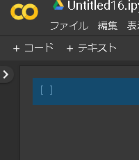

ドライブをマウント を 選択
SVMのベースモデル
from sklearn.svm import SVC
from sklearn.metrics import accuracy_score
import tensorflow as tf
import numpy as np
import pandas as pd

#GPUの利用 keras用だったはず 故にいらない。
config = tf.ConfigProto()
config.gpu_options.per_process_gpu_memory_fraction = 0.8
sess = tf.Session(config=config)
K.set_session(sess)

データの前処理パートがここに入る

Answer to the Ultimate Question of Life, the Universe, and Everything
=42
だからrandom_state=42となる。

clf = SVC(kernel='linear', random_state=42, gamma='scale')
clf.fit(X_train,y_train)
y_pred = clf.predict(X_test)

print(accuracy_score(y_test,y_pred))
########################################################################
#####SVC grid
########################################################################
Cs = [0.0001,0.01,0.1,1,10]
gammas = [0.0001,0.01,0.1,1,10]
param_grid = dict(svc__gamma=gammas, svc__C=Cs)
cv = StratifiedShuffleSplit(n_splits=5, test_size=0.2, random_state=42)
#cv=10

svm_set = Pipeline([('scaler', StandardScaler()),('svc',SVC())])
grid = GridSearchCV(svm_set, param_grid=param_grid, cv=cv)

grid_result = grid.fit(X, y)
print("Best: %f param %s" % (grid_result.best_score_, grid_result.best_params_))

grid_result = grid.fit(X_test, y_test)
print("Best: %f param %s" % (grid_result.best_score_, grid_result.best_params_))

result_dic = grid_result.best_params_
svc__C_value =  result_dic["svc__C"]
svc__gamma_value =  result_dic["svc__gamma"]


clf = SVC(kernel='linear', random_state=42, gamma=svc__gamma_value,probability=True,C=svc__C_value)
clf.fit(X, y)
df_test = df_test.fillna(0)
predict_data = clf.predict(df_test)

predict_data = pd.DataFrame({'Survived':predict_data})
predict_data = pd.concat([df_pre, predict_data], axis=1,sort=True)
predict_data.to_csv('grid_Submission1.csv',index=False)

########################################################################
#####SVC
########################################################################
X_train, X_test, y_train, y_test = train_test_split(X, y, test_size=0.3, random_state=0)

clf = SVC(kernel='linear', random_state=30, gamma='scale',probability=True)
clf.fit(X_train, y_train)
predict_data = clf.predict(X_test)
print("accuracy_score :", accuracy_score(y_test, predict_data), precision_score(y_test, predict_data), recall_score(y_test, predict_data))
print("accuracy_score :", accuracy_score(y_test, predict_data,normalize=False))
print("accuracy_score :", accuracy_score(y_test, predict_data,normalize=True))


predict_data = clf.predict(df_test)

predict_data = pd.DataFrame({'Survived':predict_data})
predict_data = pd.concat([df_pre, predict_data], axis=1,sort=True)
predict_data.to_csv('Submission1.csv',index=False)
mapとsplitの使用例のメモ
#https://www.kaggle.com/c/ieee-fraud-detection/discussion/100499

emails = {'gmail': 'google', 'att.net': 'att', 'twc.com': 'spectrum', 'scranton.edu': 'other', 'optonline.net': 'other', 'hotmail.co.uk': 'microsoft', 'comcast.net': 'other', 'yahoo.com.mx': 'yahoo', 'yahoo.fr': 'yahoo', 'yahoo.es': 'yahoo', 'charter.net': 'spectrum', 'live.com': 'microsoft', 'aim.com': 'aol', 'hotmail.de': 'microsoft', 'centurylink.net': 'centurylink', 'gmail.com': 'google', 'me.com': 'apple', 'earthlink.net': 'other', 'gmx.de': 'other', 'web.de': 'other', 'cfl.rr.com': 'other', 'hotmail.com': 'microsoft', 'protonmail.com': 'other', 'hotmail.fr': 'microsoft', 'windstream.net': 'other', 'outlook.es': 'microsoft', 'yahoo.co.jp': 'yahoo', 'yahoo.de': 'yahoo', 'servicios-ta.com': 'other', 'netzero.net': 'other', 'suddenlink.net': 'other', 'roadrunner.com': 'other', 'sc.rr.com': 'other', 'live.fr': 'microsoft', 'verizon.net': 'yahoo', 'msn.com': 'microsoft', 'q.com': 'centurylink', 'prodigy.net.mx': 'att', 'frontier.com': 'yahoo', 'anonymous.com': 'other', 'rocketmail.com': 'yahoo', 'sbcglobal.net': 'att', 'frontiernet.net': 'yahoo', 'ymail.com': 'yahoo', 'outlook.com': 'microsoft', 'mail.com': 'other', 'bellsouth.net': 'other', 'embarqmail.com': 'centurylink', 'cableone.net': 'other', 'hotmail.es': 'microsoft', 'mac.com': 'apple', 'yahoo.co.uk': 'yahoo', 'netzero.com': 'other', 'yahoo.com': 'yahoo', 'live.com.mx': 'microsoft', 'ptd.net': 'other', 'cox.net': 'other', 'aol.com': 'aol', 'juno.com': 'other', 'icloud.com': 'apple'}
us_emails = ['gmail', 'net', 'edu']
for c in ['P_emaildomain', 'R_emaildomain']:
    train[c + '_bin'] = train[c].map(emails)
    test[c + '_bin'] = test[c].map(emails)

    train[c + '_suffix'] = train[c].map(lambda x: str(x).split('.')[-1])
    test[c + '_suffix'] = test[c].map(lambda x: str(x).split('.')[-1])

    train[c + '_suffix'] = train[c + '_suffix'].map(lambda x: x if str(x) not in us_emails else 'us')
    test[c + '_suffix'] = test[c + '_suffix'].map(lambda x: x if str(x) not in us_emails else 'us')
KNNモデル 10分割交差検証+optuna
標本=分類したいもの。
AかBかにクラス分けする時に、標本を中心に円を書く。
その際に、標本が、たくさんAの円の中にあったらAに分類。
円の大きさを変えると、Bになるかもしれない。
分類の最適値がある。
import numpy as np

import pandas as pd

import matplotlib.pyplot as plt

import seaborn as sns

import optuna

from sklearn.preprocessing import StandardScaler

pip install optuna

from sklearn.datasets import load_iris

from sklearn.model_selection import train_test_split

from sklearn.neighbors import KNeighborsClassifier

from sklearn.model_selection import cross_val_score

from sklearn.metrics import accuracy_score

%matplotlib inline

iris = load_iris()
iris.data.shape

print(iris.DESCR)

df = pd.DataFrame(iris.data, columns=iris.feature_names)
df['target'] = iris.target
df.loc[df['target'] == 0, 'target'] = "Iris-Setosa"
df.loc[df['target'] == 1, 'target'] = "Iris-Versicolor"
df.loc[df['target'] == 2, 'target'] = "Iris-Virginica"

df.describe()
sns.pairplot(df, hue="target")
print(df.columns)

df.head(5)

y = df.target
X = df.drop('target', axis=1)

(X_train,X_test,y_train,y_test) = train_test_split(X, y, test_size=0.3, random_state=42)

n_train = int(X_train.shape[0] * 0.75)
X_train, X_val = X_train[:n_train], X_train[n_train:]
y_train, y_val = y_train[:n_train], y_train[n_train:]

# 標準化
scaler = StandardScaler()
X_train = scaler.fit_transform(X_train)
X_val = scaler.transform(X_val)
X_test = scaler.transform(X_test)

# 目的関数
def objective(trial):
    # C
    weights = trial.suggest_categorical('weights', ['uniform', 'distance'])
    # epsilon
    k = trial.suggest_int('n_neighbors', 1, 20)
    # SVR
    knn = KNeighborsClassifier(n_neighbors=k,weights=weights)
    knn.fit(X_train, y_train)
    # 予測
    y_pred = knn.predict(X_val)
    return (1.0 - (accuracy_score(y_val, y_pred)))

# optuna
study = optuna.create_study()
study.optimize(objective, n_trials=100)

# 最適解
print(study.best_params)
print(study.best_value)
print(study.best_trial)


##n_neighbors=3 近くの3つの点を見て、自身が誰の仲間か判断する

knn_3 = KNeighborsClassifier(n_neighbors=3)

knn_5 = KNeighborsClassifier(n_neighbors=5)

knn_9 = KNeighborsClassifier(n_neighbors=9)

##データを10分割して、分割したデータを交差して検証して…をする

scores = cross_val_score(knn_3, X_train, y_train, cv=10)
scores.mean()
Xを目印的に大きくするが、trainデータをX_train,Y_trainとしたほうがいい場合もあり、参考文献の書き方に合わせるといい。
私は好きな名前をつけて開発を始めたため、後に面倒なことになりました。
(X_train,x_test,Y_train,y_test) = train_test_split(X, y, test_size=0.3, random_state=42)
random_stateのみを変更して、結果の平均を取る手法もある。
↑うろ覚え
cross_val_score
汎用性の検証に便利なツールであるという認識で利用。
使用メモリの削減について
データ量や処理の複雑さで、メモリ使用容量が気になる時期が必ずくるはずです。
というのが参考になります。

データ型を列ごとに確認し、該当の数値を適切な型に設定し直すイメージです。
仮想環境上で、メモリが充分に使用できない時には、データ容量を少しでも減らすために、処理上の余計な変数を、
del
したりしています。
機械学習における可視化
train['カラム名'].value_counts(dropna=False, normalize=True).head()
value_countsで指定したカラムのユニークな値を出す。
Normalizeをすると、合計が1になるように正規化した値が出る。
NaN 欠損値がある場合は、dropnaを設定して動かしてみる。
ここのtrainは取り込んだデータ(CSVなど)の名前で任意です。
合同会社ムジンケイカプロ
SEO・サイト改善・業務効率支援
成果率と検索に強いホームページ制作・運用改善のご相談を承っています。
法人クライアントとの契約多数、WEB制作会社やIT専門人材との協業、サイト保守・運用まで幅広く対応しています。
(2025年7月現在)
- ランサーズ実績:238件/評価191件(★5.0)/完了率99%/リピーター29人
- ココナラ実績:販売実績66件/評価★5.0
サイト改善・集客最適化まで、一貫してお任せいただけます。
当サイトはリンクフリーです
引用・SNSでの共有はご自由にどうぞ。事前連絡は不要ですが、もしご連絡いただければ、貴社コンテンツをご紹介できる場合もございます。